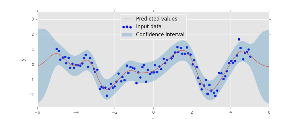
1D Kriging

An example of 1D kriging with PyKrige

import os

import numpy as np
import matplotlib.pyplot as plt

plt.style.use('ggplot')

# Data taken from https://blog.dominodatalab.com/fitting-gaussian-process-models-python/

X, y = np.array([[-5.01, 1.06], [-4.90, 0.92], [-4.82, 0.35], [-4.69, 0.49], [-4.56, 0.52],
     [-4.52, 0.12], [-4.39, 0.47], [-4.32,-0.19], [-4.19, 0.08], [-4.11,-0.19],
     [-4.00,-0.03], [-3.89,-0.03], [-3.78,-0.05], [-3.67, 0.10], [-3.59, 0.44],
     [-3.50, 0.66], [-3.39,-0.12], [-3.28, 0.45], [-3.20, 0.14], [-3.07,-0.28],
     [-3.01,-0.46], [-2.90,-0.32], [-2.77,-1.58], [-2.69,-1.44], [-2.60,-1.51],
     [-2.49,-1.50], [-2.41,-2.04], [-2.28,-1.57], [-2.19,-1.25], [-2.10,-1.50],
     [-2.00,-1.42], [-1.91,-1.10], [-1.80,-0.58], [-1.67,-1.08], [-1.61,-0.79],
     [-1.50,-1.00], [-1.37,-0.04], [-1.30,-0.54], [-1.19,-0.15], [-1.06,-0.18],
     [-0.98,-0.25], [-0.87,-1.20], [-0.78,-0.49], [-0.68,-0.83], [-0.57,-0.15],
     [-0.50, 0.00], [-0.38,-1.10], [-0.29,-0.32], [-0.18,-0.60], [-0.09,-0.49],
     [0.03 ,-0.50], [0.09 ,-0.02], [0.20 ,-0.47], [0.31 ,-0.11], [0.41 ,-0.28],
     [0.53 , 0.40], [0.61 , 0.11], [0.70 , 0.32], [0.94 , 0.42], [1.02 , 0.57],
     [1.13 , 0.82], [1.24 , 1.18], [1.30 , 0.86], [1.43 , 1.11], [1.50 , 0.74],
     [1.63 , 0.75], [1.74 , 1.15], [1.80 , 0.76], [1.93 , 0.68], [2.03 , 0.03],
     [2.12 , 0.31], [2.23 ,-0.14], [2.31 ,-0.88], [2.40 ,-1.25], [2.50 ,-1.62],
     [2.63 ,-1.37], [2.72 ,-0.99], [2.80 ,-1.92], [2.83 ,-1.94], [2.91 ,-1.32],
     [3.00 ,-1.69], [3.13 ,-1.84], [3.21 ,-2.05], [3.30 ,-1.69], [3.41 ,-0.53],
     [3.52 ,-0.55], [3.63 ,-0.92], [3.72 ,-0.76], [3.80 ,-0.41], [3.91 , 0.12],
     [4.04 , 0.25], [4.13 , 0.16], [4.24 , 0.26], [4.32 , 0.62], [4.44 , 1.69],
     [4.52 , 1.11], [4.65 , 0.36], [4.74 , 0.79], [4.84 , 0.87], [4.93 , 1.01],
     [5.02 , 0.55]]).T


from pykrige import OrdinaryKriging

X_pred = np.linspace(-6, 6, 200)

# pykrige doesn't support 1D data for now, only 2D or 3D
# adapting the 1D input to 2D
uk = OrdinaryKriging(X, np.zeros(X.shape), y, variogram_model='gaussian',)

y_pred, y_std = uk.execute('grid', X_pred, np.array([0.]))

y_pred = np.squeeze(y_pred)
y_std = np.squeeze(y_std)

fig, ax = plt.subplots(1, 1, figsize=(10, 4))
ax.scatter(X, y, s=40, label='Input data')


ax.plot(X_pred, y_pred, label='Predicted values')
ax.fill_between(X_pred, y_pred - 3*y_std, y_pred + 3*y_std, alpha=0.3, label='Confidence interval')
ax.legend(loc=9)
ax.set_xlabel('x')
ax.set_ylabel('y')
ax.set_xlim(-6, 6)
ax.set_ylim(-2.8, 3.5)
if 'CI' not in os.environ:
    # skip in continous integration
    plt.show()

Total running time of the script: ( 0 minutes 0.089 seconds)